Analysis of XML schema usage

How “big” and “complex” are real-world XML schemas?

What XSD features are used in practice and with what frequency?

Which of the known styles of schema organization are used in practice?

Our research on schema analysis started with exactly these questions.

In the present article, we lay out the results of that research: the discovered concepts of schema analysis and their application in a major study.

The article is organized as follows.

In Section 2 (“XSD metrics”), we define fundamental metrics for XSD, apply them to the schemas of the study, and interpret the obtained measures. We focus on code metrics as opposed to process metrics. The metrics are meant to facilitate certain forms of assessment, e.g., the size, the psychological complexity, or the code complexity of a schema. For instance, we have calculated bounds for the breadth and depth of XML trees, as prescribed by a given schema. We envisage that all the identified schema metrics should play a role in an improved life cycle of schemas, as means to measure trends along schema evolution.

In Section 3 (“XSD features”), we present a simple feature model of the XSD language, and we describe the corresponding schema analysis that counts feature occurrences. Technically, we simply probe whether certain XSD elements and attributes are present or not. (Only few features require more effort.) For instance, one feature inquiry may be “Does a given schema project use substitution groups or not?” Of course, such Boolean questions lend themselves to extra inquiries, as we will discuss. Again, feature analysis is meant to facilitate certain forms of assessment: dependency on the XSD language, dependency on XML-isms, and the overall complexity of the exercised feature set.

In Section 4 (“XSD styles”), we investigate the organization of schemas. That is, we attempt to determine the actual use of styles such as “Russian Doll” or “Venetian Blind”. At first sight, the results of our investigation look very promising: it turns out that most schema files adhere to one style or another. We will have to admit however that extra work is needed to make such style analysis truly meaningful. Nevertheless, it is rewarding to see that our relatively simple methodology for schema analysis allows us to make some basic concepts of schema organization very crisp – up to a point that we were able to implement a (trivial) algorithm. We call to arms for better conceptual and tool support for style management of (complex) schema projects.

In Section 5 (“XSD-isms”), we briefly discuss some XSD idiosyncrasies, relative to other data-modeling frameworks. (Some of these XSD-isms are actually XML-isms.) Our criterion for the made selection is based on our immediate interest in XML data binding, which is known to be challenged by the so-called impedance mismatch between XML (XSD) and type systems of object-oriented languages. For instance, we check for anonymous compositors. We contend that the analysis of XSD-isms is of help for decision making and impact analysis when dealing with technology choices or development options. Idiosyncrasy checking could become a best practice, to be integrated with the normal schema-development process, as to avoid late surprises.

About the schemas in the study: we have collected 63 schema projects from different sectors of IT. Some of the schemas are taken from Microsoft Webdata/XML’s internal suite of business-critical schemas that were contributed by clients of Microsoft’s XML technology. Other schemas were scanned as they were freely available on the internet. In this article, we avoid any identification of the scanned schemas; we also avoid (potentially debatable) attributions of analysis results to concrete names of schemas. The reader may assume that we made a serious effort to cover many well-known, real-world schemas, while building upon the expertise of the XML team at Microsoft. The plain schema files of the measured 63 schema projects take up 83 MB of disk space, with a median size of approximately 200 KB per project. The projects add up to approximately 6,000 individual schema files, with approximately 82,000 combined global element declarations and global complex-type definitions. The 63 projects of the study are actually only 56 distinct projects, if we do not count different versions of the same industrial schema. That is, we decided to include 3 projects with multiple versions in an attempt to gather some basic data points about schema evolution.

We will describe metrics for the size, the complexity and other properties of schemas. As usual, these metrics provide crisp quantitative measures that are meant to help with the following activities:

We begin with “comprehensive” size and complexity metrics, which summarize the size and the complexity of entire schema projects in a compressing and simplifying manner. Later, we will describe more specialized metrics, e.g., bounds for the breadth or depth of XML trees, as prescribed by a given schema. We make no claims of completeness. Software metrics is a huge field; the present paper only makes the first step to adopt this field for XML schemas, and to contribute some XSD-specific insights regarding metrics. For instance, we will not be able to report on metrics that deal with reuse, coupling or cohesion in schemas.

The calculation of schema size, in a trivial case, can be XML-agnostic. In particular, we may measure the file size of all XSD files that belong to a schema. In Figure 1, the file sizes for the schemas or the study are shown. Such a “KB metrics” is sensitive to the use of XML comments, to the average length of QNames, and to the XML indentation style. XML-agnostic (and XSD-agnostic) measures may be of limited value, but they still serve an intuitive purpose, and it is useful to identify their weaknesses anyhow.

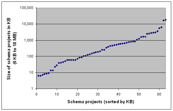
Most schemas are clearly in the range 100 KB – 1 MB (26 schemas); there also quite a few schemas in the range 10 KB – 100 KB (16 schemas); we have not found many real-world schemas with sizes below 10 KB (6 schemas); among the largest schemas, 1 MB – 18 MB, there are two schemas with multiple versions (so we may count 15 versus 11 schemas).

Figure 1. Size of schema projects in KB

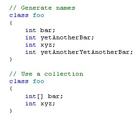
Another XML-agnostic metrics is lines of code (LOC). We note that the LOC metrics is intrinsically sensitive to line-break style and (thereby) to element-closing style. In fact, the metrics tends to miss attributes entirely. This is illustrated in Figure 2. While one may argue that attributes should count less than elements, missing them entirely is not quite favorable.

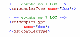
We show two (semantically) equivalent versions of the same complex type definition with quite different LOC metrics. The LOC metrics misses attributes, when common XML style is used (first encoding), i.e., when attributes are horizontally aligned next to the open tag of the hosting element.

Figure 2. Sensitivity of LOC metrics

The KB and LOC metrics are compared in a simple way in Figure 3.

Using the 63 schemas of the study as indicators, we come up with the following LOC-based categories for schema size; we also count schemas per category:

Table 1. LOC-based categorization of schemas

(There are only 3 “huge” schemas, if we do not count multiple versions.)

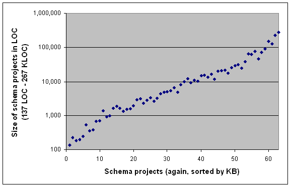
We did not sort by the primary factor, LOC, but we sorted by KB instead. Thereby the correlation between LOC and KB can be observed. The LOC measure, just as the KB measure, cannot be expected to reveal any XSD-specific insight. Both metrics just provide baseline measures for understanding the overall size category of a given schema project.

Figure 3. Size of schema projects in LOC

We become at least XML-aware now. We may simply count XML elements and attributes (not to be confused with XSD element and attribute declarations). We call this the #NODE metrics. By counting XML nodes, we immediately abstract from line-break style and element closing style. The #NODE metrics also ignores XML comments without ado (since it counts attributes and elements only, by definition). We note that the #NODE metrics still counts XSD elements for annotation; cf. documentation and appinfo. It may actually be valuable to know specifically of the amount of annotation nodes. Thus, we also provide a dedicated measure, #ANN. We summarize:

In Figure 4, we show the two measures and some of their ingredients.

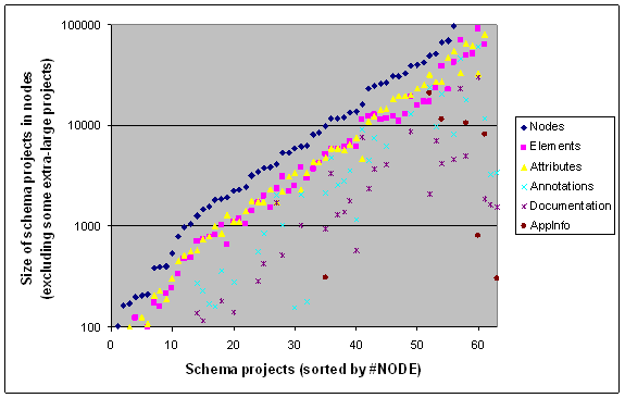
The baseline at the top shows the schema size according to the #NODE metrics; we also show the contributions of elements vs. attributes; further, we also show the amount of annotation, split up for documentation and appinfos. The ratio elements-to-attributes varies considerably. We can observe that the amount of documentation varies greatly per project. Appinfos are only used very sporadically.

Figure 4. Size of schema projects in nodes

Let us get back to the question of whether or not XML attributes should count less than XML elements. The cumulative effect of the #NODE metrics - to measure all attributes and all children of an XML element - seems to do enough justice to this issue: each XML element naturally counts as much as the content of it, while each attribute just counts as 1.

We continue exploring measures for the size of an XML schema. We become XSD-aware now; the kinds of major building blocks of schemas are counted. For comparison, for an OO programming language, we would count the number of classes, interfaces and methods. The major building blocks of schemas are global (and perhaps local) declarations and definitions. Some of these building blocks may appear to be more important than others. We discuss such calibration later.

We can easily define the following counts for global bindings:

Here are the highs and lows of these measures for the schemas in the study:

Table 2. XSD-aware counts

A side effect of this table is that we get to know about the limited usage of global model groups, attribute groups, and global attribute declarations in real-world schemas. Clearly, one should not expect any intrinsic correlation between the different categories. The actual usage of XSD abstractions very much depends on schema style and application scenario. A given schema may have more complex-type definitions than element declarations, or vice versa; it may have many simple-type definitions or (almost) none; it may use model-group definitions, or may encode all groups in complex types instead.

In an attempt to identify a single ordinal number for schema size, one may propose this sum:

Indeed, the sum of the number of global element declarations and the number of global complex type definitions is often used in informal conversations – as a common size measure for XSD. Even though we used this measure in the introduction of this paper, we want to discourage its further use because this measure is overly sensitive to XSD styles. In particular, it would not honor potentially voluminous inner element declarations as they are common in the “Russian Doll” style. Dually, we risk counting too many “types” in the case of the “Garden of Eden” style, where each global element declaration pairs up with a global type definition.

For the sake of precision, we need to consider local declarations and definitions:

… and corresponding sums:

This is still not the full set of counts. We should also define counts for references, such as element or type references. (Then, we may also need to revise some of the sums for locals+globals.) Arguably, references are not proper building blocks of schemas, but we still may need to count them for fairness. For instance, a local element declaration with a type reference to a global type should count just as much as a reference to a global element. We will miss the latter, if we do not count any references. We will count the former twice, if we do count all references. This may suggest counting only certain kinds of references for certain purposes. We are not going to engage into such “counting magic”, but we mention these issues as a justification of a simplification that follows below. The amount of possible counts is overwhelming. (Counting references is definitely of use for other schema analyses such as measuring the degree of reuse in a schema.)

We nominate the #CT measure (i.e., the sum of global and local complex-type definitions) as the primary XSD-aware metrics for schema size. Using the 63 schemas of the study as indicators, we come up with the following #CT-based categories for schema size; we also list the number of schemas that we found in these categories:

Table 3. #CT-based categorization of schemas

(There are only 8 “huge” schemas, if we do not count multiple versions.)

Clearly, #CT does not count element declarations, not even global ones. We contend that it is sufficient to count the types of all (complex-typed) element declarations. The #CT metrics is not comprehensive for other reasons; it does not honor global model group definitions, global attribute-group definitions, and global attribute declarations, neither does #CT honor simple type definitions. We contend that the #CT metrics is biased to the XML paradigm, just as much as the “number of classes” metrics is biased to the OO paradigm. We state that the #CT metrics is suggestive (“meaningful”) because:

We note that some applications of XSD may not be adequately covered by this presumption.

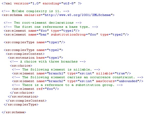
We should provide metrics that take into account XSD language concepts. To this end, we have inspired ourselves by metrics as they are used for ordinary programs. In the following, we will adopt a widely used, structural complexity metrics for (procedural) programs – the McCabe cyclomatic complexity (MCC), named after Thomas McCabe who introduced the metrics around 1976 [McCabe76]. A typical use of MCC is to approximate the psychological complexity of code, as relevant for program understanding.

There exist slight variations of the MCC definition, but an abstract characterization typically states that MCC measures the number of linearly independent paths through the control-flow graph of a program module. We may leverage existing work to adopt MCC for context-free grammars, knowing that XML schemas are grammars at some level of abstraction. That is, in [PM04], it is argued that an interpretation of MCC for grammars may simply count all “decisions” in a grammar (i.e., operators for alternatives, optional constructs and lists). We also refer the reader to [AV05] for another related effort on grammar metrics. Likewise, one may calculate MCC for procedural programs by counting all condition nodes. The comparison of grammars (or schemas) and programs makes sense in so far that the program execution of a parser, a validator, or a document processor may involve all these decisions. We presume that the process of schema understanding may also be approximated by the number of decisions.

We contend that the “important” decision nodes in XML schemas are the following:

We refer to Figure 5 for an illustration.

The various encoded decisions add up to 11 as explained in the comments.

Figure 5. MCC for XSD

In the case of normal programs, one tends to consider MCC per procedure or per module. In the case of schemas, one may also want to measure MCC at different levels of granularity. For simplicity, we immediately sum up all decisions for each schema project. Hence, we obtain a single ordinal number for the structural complexity of a schema project. This simplification is again in alignment with the cited work on grammar metrics, but a more refined approach is a valid subject for future work.

We define MCC for XSD as follows:

While the #CT metrics counts the number of named and anonymous hierarchical structuring concepts, MCC counts the number of decisions. One may say that the #CT metrics is agnostic to the use of choice as a means to introduce “subconcepts”; it is also agnostic to subtype polymorphism. The MCC metrics is exactly meant to measure those “decisions”. The MCC metrics is (deliberately) insensitive to the use of flat content models vs. the use of extra elements for grouping parts of a content model. Clearly, the #CT metrics is sensitive in this manner; see Figure 6 for an illustration.

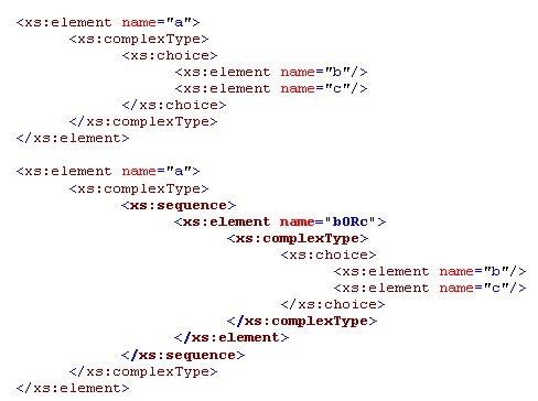
The MCC measure for these two element declarations is the same regardless of the extra subelement bORc that appears in the second version.

Figure 6. Reduced sensitivity of MCC metrics

Some details of the above definition are worth discussing.

One may argue that a choice should contribute just 1 to a schema’s MCC, regardless of the number of branches. By counting the number of branches, we honor each branch as a “decision”. An MCC metrics for imperative programs tends to count the cases of an imperative switch statement (as in C++) just like that. This argument can be adopted for substitution groups and type references. That is, MCC for XSD captures that “subtype polymorphism” introduces complexity, which increases with the number of “subtypes”.

One may argue that a singleton choice (i.e., a degenerated choice with just one branch) should not count at all.

One may also argue that each attribute with use=“optional” should contribute 1 to a schema’s MCC. However, the optional status of an attribute is the common case (in fact, optional is the default for use), which does not warrant a proper decision.

One may also argue that any attribute and any element of a simple type require a sort of “decision” in so far that the simple type must be inhabited as such (unless a default is present). We do not count these leaf-level decisions as they may lead to an explosion of the total number of decisions.

Finally, one may argue that certain or all uses of wildcards (any, anyAttribute, xs:anyType) suggest counting these wildcards in the calculation of MCC. The use of these features is however better observed in a more prominent manner than a slightly increased MCC. Use of any and friends will show up in the feature profile of a schema.

MCC correlates with XSD-agnostic schema size in so far that a larger schema is likely to comprise more decisions. However, schemas differ heavily in their amount of decisions “per node”; cf. Figure 7. (Note that the MCC measure is shown on a logarithmic scale.) This weak correlation between MCC and #NODE is of course very much appreciated because it indicates the additional information contributed by MCC. (We should engage in a scatterplot or some other means to properly investigate the correlation between MCC and #NODE, which we leave for future work.)

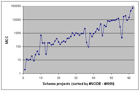
All the local peaks can be explained relatively easy by inspection of the schema in question. One will find that decision operators are heavily used: choices, substitution groups, or others. Dually, the local lows hint at a very simple direct XSD coding style for plain hierarchical organization.

Figure 7. MCC vs. the number of schema nodes

Using the 63 schemas of the study as indicators, we suggest categories for MCC-based schema complexity. To decouple ourselves (somewhat) from #NODE-based schema size, we categorize the ratio (#NODE - #ANN) / MCC:

Table 4. MCC-based categorization of schemas

The distribution of (#NODE - #ANN) / MCC for the schemas of the study is illustrated in Figure 8.

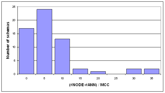
The chart provides a discrete view on the ratio (non-annotation) nodes to MCC. We have approximately 2.6 M nodes (without annotations) in the study and the accumulated MCC measure for all schemas is approximately 0.7 million, the average ratio is close to 4. That is, 1 MCC unit corresponds to 4 nodes. This concentration is also observable in the chart.

Figure 8. Ratio schema nodes to MCC

MCC is widely accepted (for procedural programs). We believe that our transcription to XSD is faithful. However, there is no doubt that MCC generally (and perhaps unduly) focuses on complexity in the sense of “decisions”. Such bias may be more useful for imperative programs than XML schemas because of XML’s focus on hierarchical organization of data. The #CT metrics pays attention to the idea of hierarchical organization in so far that it counts hierarchical concepts. In the following, we complement the #CT metrics by different kinds of breadth and depth measures.

To be more precise, for both breadth and depth, we will provide two metrics. There is a code-oriented measure, which approximates efforts in program understanding, and there is an instance-oriented measure, which approximates complexity of the resulting XML trees.

We begin with the code-oriented breadth measure for the number of parties in a content model. (We will make the term party more precise in a second.) We will aggregate a maximum breadth value (per schema) from the various breadth values for all the individual content models.

The code-oriented breadth of a content model is defined as follows:

A sample calculation is carried out in Figure 9.

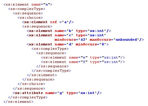
We face a global element declaration. We are interested in the code-oriented breadth of its content model. All contributing parties are highlighted. The computed breadth is 4 when excluding attributes and 5 when including attributes. The relevant parties are these: a, b, c, d, g; the latter is an “attribute” party; all the others are parties for immediate subelements; the inner elements, e and f, do not count for the content model of the root element declaration; they would rather count for the content model of the local element declaration d.

Figure 9. Code-oriented breadth

In Figure 10, we show the distribution of code-oriented breadth measures for the schemas in the study. We recall that the breadth value for a schema is simply the maximum of the breadth values for all the content models (say, complex types) in the schema.

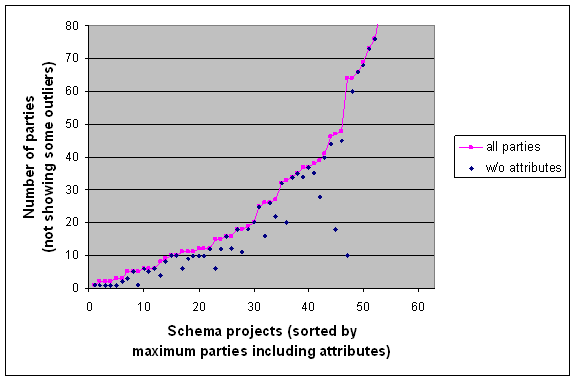
Half of the schemas in the study have at least one content model with more than 25 parties. The difference between “parties including attributes” versus “parties excluding attributes” is visually striking in at least 10 cases. These projects clearly use complex type definitions with many attribute declarations. We recall that the shown measures honor code abstraction through model groups, attribute groups and type extension. The counts would be higher, if these abstractions were dereferenced.

Figure 10. Distribution of code-oriented breadth

There are about 11 schemas in the study with a number of parties that is above 100 (not shown in the figure). This is a striking degree of complexity. We have looked into these schemas one-by-one. Normally, there is just a very small number of “monster types”, perhaps just one choice or sequence group that enumerates all defined types. There are just two schemas in our study which comprise a significant percentage of complex types (> 5%) with well above 100 parties.

We turn from code-oriented complexity to instance-oriented complexity. We say that we measure (a bound for) the number of children, again, selectively including attributes. As before, we aggregate a single breadth value for an entire schema by taking the maximum of the individual breadth values for all the content models.

The definition of instance-oriented breadth of content models is characterized as follows:

A sample calculation is carried out in Figure 11.

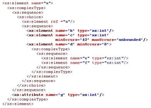
In the previous section, we calculated 5 parties for the code-oriented breadth of the sample at hand. By contrast, the instance-oriented breadth is 45 children. Again, this number includes one attribute. The contributions to 45 are emphasized in bold face; we have opted for the heavier branch of the choice, as prescribed by the above definitions.

Figure 11. Instance-oriented breadth

In Figure 12, we show the distribution of instance-oriented breadth measures for the schemas in the study.

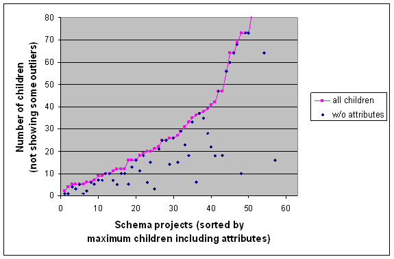
The distribution for instance-oriented breadth (this chart) is very similar to the distribution for code-oriented breadth (previous chart): half of the schemas in the study have 25 children as maximum or less. On the one hand, not each party actually contributes to the instance-oriented measure (due to choice). On the other hand, a single party may contribute several children (due to dereferenced base types, model groups, and others). These observations explain why it is possible that code-oriented and instance-oriented breadths may correlate so well as it is the case for the schemas of the study. In the chart, the contributions of attributes are again remarkable. Several schemas define large attribute groups or indeed just many individual attribute declarations.

Figure 12. Distribution of instance-oriented breadth

We will now investigate the level of nesting in content models and instances thereof. We will start with a code-oriented metrics that basically measures the nesting of constructs for content modeling. Again, this code-oriented metrics will be later complemented by an instance-oriented metrics, which will provide a bound for the level of element nesting in actual XML trees.

Code-oriented depth is defined as follows:

We refer to Figure 13 for an illustration that continues our running example.

We refer to Figure 14 for a chart with the code-oriented depth values for the schemas of the study.

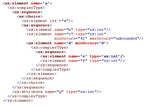
The full descriptional depth, 7, is contributed by the elements in bold face.

Figure 13. Full descriptional depth

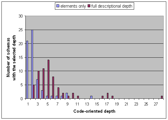
The pure nesting of element declarations is limited to 2 for the majority of content models. There is a single schema that exercises element nesting up to the level of 14. The full descriptional depth is systematically greater, as one would expect.

Figure 14. Distribution of code-oriented depth

We also want to measure the height of XML trees, as prescribed by element declarations and their content models. The most obvious approach to an instance-oriented depth measure is to define the greatest lower bound (glb) on the depth of XML trees that are derivable from a given root-element declaration. By the depth of an XML tree we simply mean the longest path from the root to a leaf, while counting each element tag along the way. Given a root element declaration r, we say that n is the glb-depth of r, if (i) all valid instances of r have a depth of n or more, and (ii) there is at least one valid instance of depth n. The glb-depth of a schema could be calculated by a folk-lore fixpoint algorithm.

However, there are some problems with this innocent mathematical concept:

There is no valid instance for this root-element declaration.

Figure 15. Recursion without proper base case

Recursion does not terminate without the minOccurs constraint.

Figure 16. Recursion with optionality-based base case

We have addressed the aforementioned problem by a dedicated fix-point algorithm, which starts from the basic glb algorithm, and ignores all minOccurs=“0” constraints “as long as possible”. In the course, of fix-point computation, more and more root element declarations and global complex-type definitions are associated with finite depth values. Once fix-point computation stops to make progress, we let it “cease”, i.e., we take minOccurs=“0” constraints into account so that additional finite depth values can be obtained. This is an ad-hoc solution, which needs to be justified, complemented and formally described in future work.

For comparison, we compute two values:

Our measurements are shown in Figure 17.

The running example is continued in Figure 18.

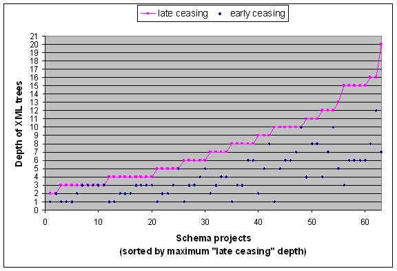
Approximately half of all schemas define a maximum depth greater than 7. Even with early ceasing, there are a good number of schemas with a maximum depth greater than 5. We can clearly see that we get much smaller depth values if we just apply the glb-depth algorithm.

Figure 17. Distribution of instance-oriented depth

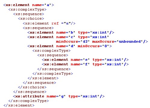
We emphasize the parts of the original element declaration that would contribute to an XML tree of the computed depth, for the case of late ceasing. Hence, the value for late ceasing is 3. For early ceasing, the optional element d will not be counted.

Figure 18. Instance-oriented depth

One may argue that breadth and depth measures should be combined in a kind of “volume” measure. In the instance-oriented version, one may think of volume as a bound for the number of XML element nodes in an XML instance that serves as the shortest valid completion from a root element tag. Purdom’s folklore algorithm for shortest completion of nonterminals in a context-free grammar [Purdom72] would need to be adopted for XSD. We view volume metrics and other elaborations of depth and breadth measures as topics for future work.

We turn to a different subject: XSD features and the analysis of their usage. Essentially, we use the term feature to refer to an XSD language concept for which we can probe by checking whether or not certain XML elements and attributes (of the XML Schema namespace) occur. For a quick overview, we provide a feature matrix that is spread over Figure 19 and Figure 20.

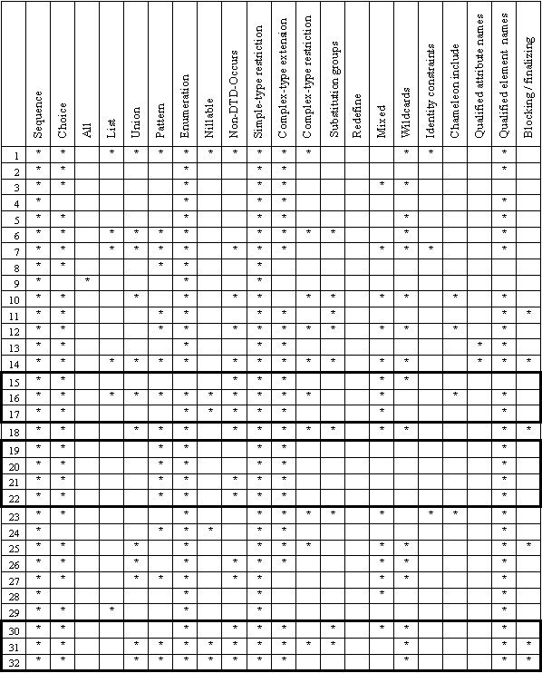
We highlight 3 clusters that comprise multiple versions of the same overall schema project.

Figure 19. Schema features – part 1

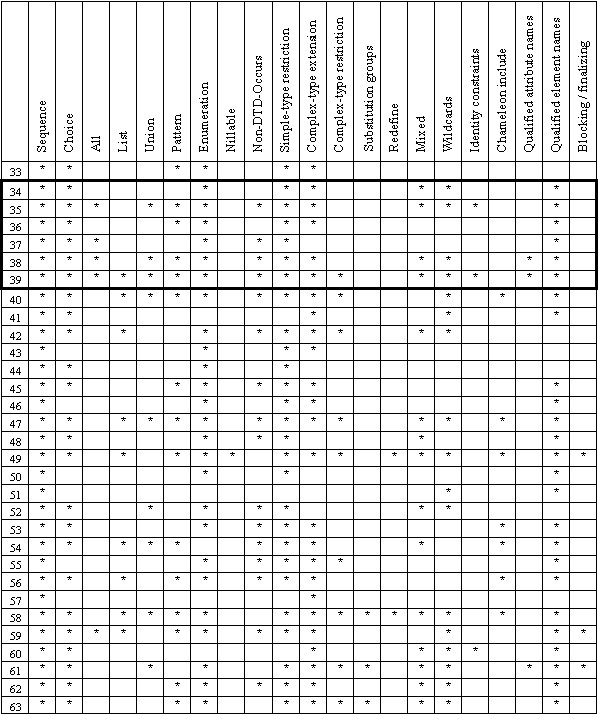
We highlight the family of MS Office schemas. The family members commit to quite different feature sets.

Figure 20. Schema features – part 2

In Figure 19, we highlight some clusters that comprise multiple versions of the same overall schema project, shown in the order of releases. These are two large schemas and one huge schema, according to our LOC-based categories. Cluster I: the initial version (schema 15) used a small feature set; the 2nd version (schema 16) went very much beyond it; the latest version (schema 17) is cut back again with regard to the exercised feature set. Cluster II: all four versions, schemas 19 – 22, use the same small, almost DTD-like feature set, except that later versions started to use identity constraints and nillable elements.

In the following subsections, we discuss many features in detail. We will present a “schema count” per feature (i.e., the number of schemas of the study that use the feature in question) and a “total count” (i.e., the total number of feature occurrences in all schemas of the study). Where useful, we also list some additional features that did not fit into the feature matrix. In several cases, we will also offer a “censored count”, whenever we have reason to believe that the total feature count is skewed by just a few outliers. (Normally, we only allow ourselves 1 or 2 outliers. Several counts are indeed skewed by the fact that some schemas seem to be generated by tools in a somewhat non-idomatic way.)

Table 5. Model group operators

Not surprisingly, all schemas use sequences. The typical ratio sequences to choices is 10 : 1. There is a single, medium-sized schema that uses 14,655 choices alone. (Inspection reveals that the bulk of these choices is degenerated, i.e., there is a single branch per choice only. One may suspect that the schema was generated.) “Alls” are used only very sporadically. There is a single, small schema that uses 23 alls out of 40 (total count) alone.

Table 6. Simple type features

The number of simple-type restrictions coincides, by definition, with the number of simple type definitions that use facets. (We recall that a simple-type definition boils down to either a restriction, or to a list type, or to a union type.) To provide additional data, we mention that there are 12,410 simple type definitions versus 62,168 complex-type definitions in our schema base. Hence, we can report that the ratio simple-type to complex-type definitions is 1:5. Lists are not widely used – according to the table, which may be explained by known limitations for processing lists (cf. lack of XPath expressiveness for lists). Facets are used 20 times more often than unions, if we consider the censored count for unions (1 outlier).

The intensive use of enumerations suggests that they need to be seriously supported by XSD technologies. For instance, XML data-binding technologies vary considerably with regard to support of enumerations. 3 schemas (outliers) use much more than half of enumeration constants. Inspection reveals that these 3 schemas define voluminous enumerations with hundreds of enumeration constants. Once we take these schemas out of the equation, we can determine an average size of 10 enumeration constants per enumeration.

The relatively small amount of patterns is perhaps surprising, especially when we note that approximately 800 out of 925 feature occurrences are contributed by 4 schemas alone.

Our analyses are by no means complete. We look forward to future work on the subject. Just to give an example that is related to simple types, one may also be interested in the use and the number of occurrences for the various primitive simple types. In particular, it will be interesting to see how legacy types (such as ID and IDREF) are used, if at all.

For the lack of a better term, we use the category “occurrence” features for all those features that deal with presence, absence or multiplicity of elements or attributes. The minOccurs and maxOccurs constraints most obviously belong to this category.

Table 7. Occurrence features

In the feature matrix, we showed the fact whether or not a schema uses “non-DTD occurs”. By this we mean all combinations of explicit or default attribute values for minOccurs and maxOccurs that cannot be expressed directly through DTD operators *, +, ?. All the possible forms of “DTD occurs” are these:

Before censoring, close to 10% of all occurs are non-DTD occurs. However, 3 schemas (in fact, 2, if we eliminate multiple versions) use most of these non-DTD occurs. After censoring, only 0.5% of all occurs go beyond DTD.

The huge total count of nillables originates from 3 schemas (in fact, 2, if we eliminate multiple versions). The schemas in question seem to be generated, and the template seems to be such that every element is allowed to be nillable. There are only 7 nillables left for all other schemas. We contend that the nillable feature may be overrated.

The use of the attributes fixed and default suggests that these features are widely used. We have not checked on the distribution over element versus attribute declarations.

We have found 7,866 attribute declarations with use=“required”, which is about 10% of all attribute declarations. This suggests that schema designers predominantly use attributes for optional data parts (as opposed to required ones). We have only found very few uses of use=“prohibited”. We recall that this feature is used when an attribute should be “restricted away” in complex-type derivation by restriction. There are 1,061 occurrences of such type restrictions in the schemas of the study, but only 24 cases of prohibition. So the feature should not be overrated.

The last row of the table shows the amount of “unnecessary XSD attributes”, i.e., attributes, where the specified value coincides with the default value for this XSD attribute, prescribed by XSD – such as in use=“optional”. There are 1.8 million attributes in the schemas of the study; before censoring, one out of six attributes is unnecessary; censoring reduces this number by factor 10.

For the lack of a better categorization, we group a few features that all relate to XSD’s different forms of subtyping. (We had listed simple type restrictions earlier already, but we repeat them here for comparison with complex-type derivation.)

Table 8. Subtyping features

The total count for substitution groups lists substitution bases only (as opposed to the total number of participants in substitution groups). By contrast, all the total counts for type derivation list the actual number of type extensions and restrictions. Nevertheless, the schema counts unambiguously indicate that complex-type subtyping (“extension”) is by far more commonly used than element subtyping (“substitution groups”). This is well in line with common recommendations that disfavor substitution groups. We may also look at the situation for the three clusters for which we have several schema versions; see the feature matrix. Two of the projects have never used substitution groups. The third project has (very recently) eradicated element subtyping in the latest version.

Complex-type restriction (with complex content) is modestly used in our schema base – complex-type extension is used 10 times more often. It turns out that complex-type restriction with simple content is used only very sporadically.

XML technology providers have been struggling with the correct implementation of REDEFINEs. However, there are only two medium-sized schemas (according to our LOC-based categories) in the study that actually use this feature. Apparently, no schema owner of a large or a huge schema takes the risk of a dependency on a feature that is still unimplemented or incorrectly implemented by some technologies.

We have measured blocking and finalization (for subtyping) by checking for the schema attributes blockDefault and finalDefault as well as for the attributes block and final on element declarations and type definitions. The corresponding counts clearly indicate that schemas are kept very “open” for extension (and restriction). We wonder whether all this unblocked and non-finalized subtyping is intended and desirable.

Table 9. Mixed content

Half of all schemas use mixed content.

We note that we measure mixed content simply by means of testing for the attribute mixed. It is a well-known fact that many schemas use string-typed content models for storing text in elements. Unfortunately, we cannot determine such cases of mixed content without precise knowledge of each and every schema. We also note that one may want to add further measures regarding mixed content, such as the ratio of mixed content models vs. non-mixed content models in a schema. Given, the relatively small number of occurrences of mixed and the huge number of complex-type definitions, it is clear that mixed content models constitute a very small minority.

Table 10. Extensibility

Half of all schemas use wildcards (to define extensibility points, of for other reasons). The table also shows the distribution for the different namespace constraints on wildcards. It turns out that two forms are never used, and the URL form is used only sporadically.

Table 11. Identity constraints

Identity constraints are used sporadically.

Most of the schemas in the study (namely 47) consist of multiple files. The combined number of all schema files in the study is 5,970. This gives rise to the examination of modularization features.

Table 12. Modularization

A third of all schemas in the study contain one or more files that do not define a target namespace. Several of these schemas though are one-file projects: 9 out of 20. The remaining 11 schemas actually use Chameleon includes (i.e., the bindings of the included file adopt the target namespace of the including file). Also, there are only 9 out of the 47 multi-file schemas that use both includes and imports; the remainder either uses includes or imports alone. The measurements indicate that includes are preferred over imports. However, there are 3 schemas with thousands of smallish files that are composed through includes. When these schemas are taken out of the equation, then there are just twice as many includes as there are imports.

A general note on schema modules is in place. For many of the larger or huge schema projects, we could guess from background knowledge and from the directory structure, that some internal modularization is present. We were particularly interested in the question of whether or not to split up some of these schema projects into several smaller schema projects so that we would obtain more data points; so that we would not confuse independent parts. However, we could not easily establish a uniform and robust way of taking schema projects apart. For instance, there is often an overlap of inclusion, which defeates any attempt of partitioning the files that belong to a given project. Some projects use a flat directory structure, even though some clusters seem to exist. Also, the identification of proper “root files” is not always straightforward. For instance, several schema projects comprise hundreds of entry points, e.g., files for the many “business transactions” that are modeled. However, this granularity is not suitable for the identification of smaller schema projects to be distinguished in our analyses. We conclude that we lack a simple and generic approach to the identification of sub-project structure in multi-file schema projects.

We will now look at styles for “schema organization”, such as “Russian Doll” and “Salami Slice”. These styles are documented in the XSD literature and discussed in various online resources [Maler02], [XSD]. In the context of schema analysis, it is natural to wonder whether we can probe for the styles, and whether we can quantify their potentially inconsistent use. We recall these folklore styles briefly, while we ignore all namespace considerations that may be relevant for a deep understanding of the styles:

One may formally specify these styles in terms of the XSD-aware counts that we have defined earlier. The following matrix defines the styles by reference to #ELg (number of global element declarations), #CTg (number of global complex-type definitions), #ELl (number of local element declarations), #CTl (number of local complex-type definitions), and #ELr (number of element references).

Table 13. Schema styles (strict)

(An empty cell means that the number is unconstrained: “>= 0”.)

Our specifications are readily useful to make some crisp observations. The folklore styles seem to ban the combined use of local element declarations and element references. Dually, the folklore styles seem to ban the combined use of global and local complex-type definitions. In both cases, we want to argue that the added permission for local abstractions should not be considered bad style or “non-styled”. Adopting programming-language insights, we claim that the use of locals for an existing category of abstractions is just an instance of “information hiding”. There are little reasons other than syntactic or religious ones not to allow for the following relaxed styles:

Table 14. Schema styles (relaxed)

We should note that our discussion does not rely on these relaxations; we merely want to offer them for discussion. There is no relaxed form of the “Russian Doll” style simply because "matryoshka" is already perfectionist in information hiding. We also note that the relaxed form of “Garden of Eden” is very liberal indeed: locals of both kinds can be incorporated while none of them was admitted by the strict form. We presume that there are likely to exist other ways for deriving a comprehensive set of styles, but we stop here with this investigation.

One may say that every scenario that is not covered by the folklore styles (or some relaxations thereof – like ours) should be considered non-styled. Both labels about stylishness and non-stylishness may be incorrect, given the simplifying nature of our definitions. One potential problem is that our definitions do not constrain the use of includes and imports. Another potential problem with the above specification is that it ignores some forms of XSD abstractions. For instance, simple-type definitions are not measured. This observation suggests the following special category:

Table 15. “No trees” schema style

“No trees” deals with schemas (files) that are not even meant to define types of tree-shaped instance data. Schema files that specialize in simple-type definitions belong to this special category.

We have measured the adherence to style in the schemas of the study. To this end, we have assumed that each individual file is tested for a coherent style. We are prepared to find that different files of a schema project may vary in style. Ultimately, we want to know the degree of styling. Here are the results:

As a simple way to digest some of these numbers, we recall that the calculation of the code-oriented depth measure revealed small values for the element-nesting depth of most schemas. This fits with the small number of files in the “Russian Doll” style. Here we note that the element-nesting depth for the other (strict) styles is intrinsically limited to 2.

Given the fact that contemporary schema design tools do not directly help the schema developer with maintaining a certain style, it is perhaps surprising to see that more than half of all schema files are strictly styled. (By this we mean that all the individual files in a project adhere to one strict style or another.) However, there are only 4 schemas in the study that are consistently (strictly) styled, and these are, without exception, small or monolithic schemas. (We say that a schema project is consistently styled, if all files of the project adhere to the same style.) Most schemas are mix-styled and it is s not exactly clear how to judge these cases. There are presumably some forms of mixing and some potential intensions for mixing that are laudable, but we lack knowledge of these forms and we do not have access to project-specific intentions. It is also very likely that the different styles reflect, to some extent, the fact that (large) schema projects are developed by several people who lack an effective way of agreement on style and enforcement thereof.

At the file level, it is actually not particularly difficult to be styled. One can see this by carrying out a simple combinatorial inspection of the coefficients in our specification. Being styled is even easier, once we take (reasonable) relaxations into account. Our carefully proposed set of relaxations immediately provides us with 84.71% of (relaxed) styled files. The key question seems to be then whether a certain style was intended and whether the styles per file in a schema project add up to a useful style of the entire project. We note that our style analysis is purely local and syntactical; it does not constrain the composition of the complete schema from its individual components; nor does it constrain the actual idiomatic details of type and element references. For instance, it may be that a given file (accidentally) exposes a strict style by itself, but all includes or imports of this file lead to a non-styled composition. So we really need to attach a major disclaimer to the kind of style analysis that we have described so far:

Much more work is needed to deal faithfully with XSD styles.

We have also looked at the three schemas for which we have multiple versions available. Strong stylishness gets gradually lost along the evolution of all these three schemas. We can only hypothesize that this may indicate modifications of the schemas that were carried out by different people in the absence of an explicit and tool-enforced profile for the style of the projects.

We view the following discussion as an application of our generic methodology for schema analysis – an application that has an immediate benefit for XML technology such as tools for XML-to-object or XML-to-relational mappings. We will look into XSD idioms (or rather “XSD-isms”, some of them being “XML-isms” in fact) of the kind that set XSD apart from other data modeling languages, and (or) that make it more challenging to map XML schemas to other paradigms or languages. Given the complexity of the subject (and the expected word count of this publication), we will only touch on this topic.

When model groups are nested in XSD, then there is no name-based way to address the inner compositor; cf. Figure 21 for an illustration. This may be a problem when mapping those data-model patterns to the object-oriented paradigm, as it is done in XML data binding (aka XML-to-object mapping). It is then necessary to improvise as follows; either (i) we give up on grouping in the target data model, or (ii) we generate names for anonymous compositors; cf. Figure 22 for some potential mapping results, shown in C# syntax.

The inner choice is anonymous.

Figure 21. Anonymous compositors

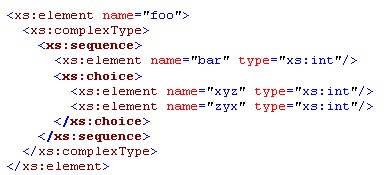
We show two options for mapping the anonymous choice from Figure 21.

Figure 22. Mapping anonymous compositors

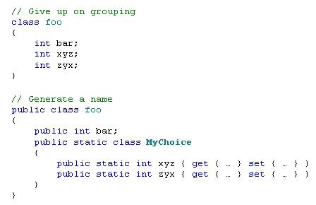
A particularly strong version of anonymous composition is present when grouping also involves occurrence constraints; cf. Figure 23 for an example. The trouble is that (i) “giving up on grouping” would boil down to two divorced (hard to sync) lists; and (ii) “name generation” is just as inconvenient because we may need two generated names at once: the name for the item type and the name for the list field.

In need of names - we may want to address the inner list of pairs and each single pair.

Figure 23. Strongly anonymous compositors

Our measures indicate that anonymous compositors are used quite heavily:

Table 16. Frequency of anonymous compositors

The censored count is based on the exclusion of 4 schema projects (not counting multiple versions). This is the most aggressive (and thereby debatable) claim about outliers in this paper. One of the outliers is a project that skewed several other counts. Yet another of the outliers is a legacy version of a schema project with multiple versions. The remaining two outliers are important schemas that use many anonymous compositors both in previous and in current versions. So no matter what, anonymous compositors constitute a practically relevant XSD-ism.

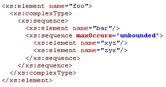
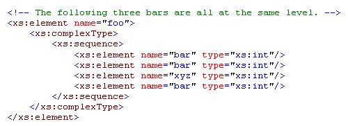
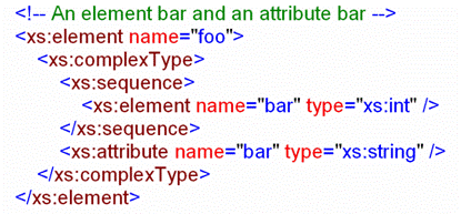
Another known friction issue for XML data binding is the potential of multiple occurrences of an element name in the same content model; cf. Figure 24 for an illustration. From an XML/XSD-centric point of view, there is absolutely nothing wrong with this use of element names. The point is that element names are nothing but node labels, even though we may want to think of them as subtree selectors. To resolve this impedance mismatch, XML data binding will have to engage in “name mangling”. Another option is to map the offending element name to an array (or an indexed property). Both options are illustrated in Figure 25.

XSD element names are not exactly meant to be selectors. They are node tags.

Figure 24. Recurring element names in a content model

The illustrated techniques manifest an impedance mismatch. For instance, the second solution is suboptimal in so far that the use of an array (likewise for an indexed property) is not totally safe. One has to be careful to observe that indexes 0..2 are valid only. Also, the XSD order constraint (bar, bar, xyz, bar) is not discoverable for the OO programmer.

Figure 25. Map recurring element names

We will list counts for ambigious selectors in a single, comprehensive table at the end of the section.

XSD defines separate symbol namespaces (not to be confused with XML namespaces) for various sorts of symbols that may be declared or defined in a schema. In Figure 26, we show a trivial example that inhabits the symbol namespaces for elements and types with the same lexical name. In Figure 27, we show that this problem is also relevant for local names in content models. When mapping schemas, the target domain is not likely to offer the same sort of symbol namespaces, which again implies the need for “name mangling”.

The two foos live in different symbol namespaces.

Figure 26. Name collision (global bindings)

The shown code fragment shows the simplest situation. In practice, the “conflicting” name occurrences may be visually divorced due to model-group references and type derivation by extension.

Figure 27. Name collision (elements and attributes)

We will list counts for collisions due to symbol namespaces in a single, comprehensive table at the end of the section.

Another friction issue concerns the fact that XSD is case-sensitive, while the target domain of data-model mapping may be case-insensitive or at least less case-sensitive, which may lead to a situation where names that are different in XSD are considered the same in the target domain. So again, name collisions may occur, which have to be resolved through name mangling.

We summarise counts for several XSD-isms in the following table.

Table 17. Potential XML data binding issues

The table clarifies that case sensitivity and symbol namespaces are exploited in real-world XML schemas; more generally: all kinds of name collision issues are real-world problems. It turns out that, by average, each schema project would face a bit less than 100 friction issues, before censoring. 2 schemas alone account for nine tenth of all ambigious selectors, where one of these schemas is obsolete by now (i.e., it has already been replaced by a new version). The censored number of friction issues is still too large to be ignored.

We have researched the topic of quantitative and qualitative XML schema analysis, while our motivation was a better understanding of real-world XML schema usage and the provision of methods that help monitoring the status of schema assets along development and evolution. We have developed all necessary concepts of XML schema analysis, we have executed a detailed empirical study of schema usage, and we have reported all important results. At the conceptual level, we have introduced fundamental metrics for the XSD language, and we have identified the basic feature model of the XSD language. At a more problem-specific level, we have looked into issues that are related to the so-called impedance mismatch in data-model mapping, as it is relevant for XML data binding.

There is one very obvious topic that we have circumvented in the present paper: large-scale analysis of instance data while feeding back the results of these analyses into schema-level problems. Most notably, one may be interested in coverage analysis. (What part of the schema is actually exercised by all the available instance data?) Such coverage measures could be used to steer simplifications of a given schema on the basis of the existing data harness. The conclusive analysis of instance data with subsequent applicability to schema-level problems (such as schema simplification) necessitates the availability of substantial real-world data. (For some interpretations, one even may want to have access to all existing instance data for the schema in question.) For the exact schemas of the study, we do not have access to such a harness of instance data, but we support that work on instance-data analysis is an important complement of our efforts.

To summarize, schema analysis is a key ingredient of an emerging engineering discipline for XML schemaware, schema-based data management, schema-aware XML programming, and more generally: software development that includes XML schema artefacts. We expect that schema analysis of metrics, features, styles, and others becomes an integral part of XML schema-development processes, on the basis of appropriate tool support. We envisage that the future schema developer can easily observe trends for schema metrics along development. Also, the schema developer is enabled to express intentions about complexity, features and styles so that warnings can be produced timely by the schema editor, when the intentions are about to be violated.

We are grateful for discussions with other members of the Webdata/XML team at Microsoft, while we mention Dan Doris and Priya Lakshminarayanan in particular. Special gratitude is due to our team member Zafar Abbas for his help with the schema base of this study complete with general XSD expertise. Further, we acknowledge interaction with James Power (National University of Ireland) and Brian Malloy (Clemson University) whose paper on grammar metrics [PM04] proved to be inspirational for some of our efforts on XML schema analysis.

[AV05]

Tiago Alves and Joost Visser: Metrication of SDF Grammars, Technical Report, Departamento de Informática, Universidade do Minho, DI-PURe-05.05.01, May 2005, also see the SdfMetz, website http://wiki.di.uminho.pt/wiki/bin/view/PURe/SdfMetz for additional information.

[Maler02]

Eve Maler: Schema Design Rules for UBL...and Maybe for You, XML Conference & Exposition 2002 (XML’02), See http://www.idealliance.org/papers/xml02/dx_xml02/papers/05-01-02/05-01-02.html for the online proceedings.

[XSD]

For the readers convenience, we link to a number of not necessarily peer-reviewed resources about schema organization, schema styles and schema coding practices: http://www.xfront.com/GlobalVersusLocal.html; http://lists.xml.org/archives/xml-dev/200010/msg00770.html; http://devresource.hp.com/drc/resources/xmlSchemaBestPractices.jsp; http://www.dcs.bbk.ac.uk/~ptw/teaching/schemas/notes.html; http://xml.sys-con.com/read/40580.htm

[McCabe76]

T.J. McCabe: A Measure of Complexity. IEEE Transactions on Software Engineering, 2(4), pp. 308-320, December 1976. See http://www.sei.cmu.edu/str/descriptions/cyclomatic.html for a high profile online resource on the McCabe metrics. See http://www.verifysoft.com/en_mccabe_metrics for another one. Online resources are mentioned here for the convenience of the reader of the present article.

[PM04]

J.F. Power and B.A. Malloy: A metrics suite for grammar-based software, Journal of Software Maintenance and Evolution, John Wiley & Sons, Inc., 16(6), 2004, pp. 405-426.

[Purdom72]

P. Purdom: A sentence generator for testing parsers. 1972, BIT 12, 3, 366–375.

Biography